Introduction
Over the past decade, one of the bigger mysteries in the field of deep learning has been why certain massively overparametrized architectures generalize so well. While the standard gospel of machine learning preaches the bias-variance tradeoff and the dangers of overfitting our models to the training data, many large neural architectures display behavior contrary to this.
For example, as we increase the number of parameters of a standard neural network (a
multilayer perceptron), its model capacity grows, and it initially displays behavior
similar to the traditional bias-variance curve, shown in Figure 1(a). Eventually, the
model capacity becomes large enough that the network can fit the training data
exactly. At this point, called the interpolation threshold in Figure 1(b), standard
bias-variance theory tells us we should expect our model to have drastically overfit the
training data, so that its performance on test data will be poor. But if we increase the
model capacity even further, we observe something strange: the test error starts to
decrease again, as shown in Figure 1(b).
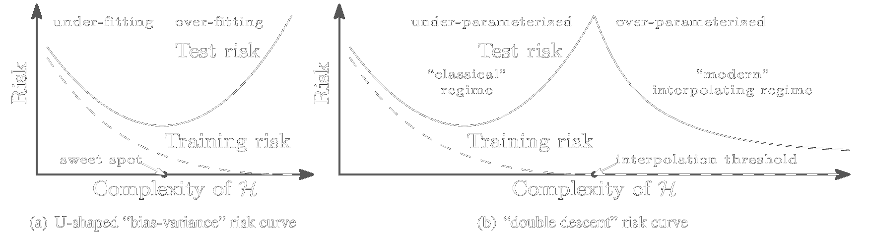
Figure 1: a) The classical bias-variance tradeoff. b) The behavior for overparameterized neural networks. Taken from Belkin et al. (2018).
This behavior in overparameterized networks was first seen empirically, so one might
wonder if we can set up a situation where we can see this behavior analytically. One
interesting regime is the limit where the network layer widths go to infinity, which
corresponds to the far right end of Figure 1(b). This sort of infinite limit is often
used in physics, as it makes certain analyses analytically tractable. For example,
thermodynamics emerges from statistical mechanics in the limit where the number of
particles goes to infinity. The hope is that in the infinite limit, a) some
non-trivial behavior of the finite-sized system remains, and b) the study of this
behavior will yield to analytic analysis.
The infinite-width limit was studied in Neal (1994), where it was shown that a network with a single hidden layer behaves as a Gaussian process when the hidden layer width goes to infinity. In Lee et al. (2017), this result was extended to networks with an arbitrary number of layers, introducing the concept of a neural network Gaussian process (NNGP). A Gaussian process is a method for doing Bayesian inference, and an NNGP is a way of doing Bayesian inference with neural networks (in this case, for regression), and obtaining error bounds for the predictions. This is in contrast to the standard method of training neural networks with gradient descent on maximum likelihood, which does not provide error bounds.
It’s important to clarify that this analysis only applies to a special, seemingly restricted case: the behavior of the infinite-width network at initialization. In particular, if we wish to compare the performance of a NNGP to a finite-but-large-width network trained via gradient descent, we only train the network weights between the final hidden layer and the outputs. The rest of the weights are frozen at their initialization values. Surprisingly, this sort of minimally trained network has non-trivial predictive ability.
The details of the NNGP calculation can be confusing — at least they were for me — so the aim of the rest of this post is to make these details clear. I’ll assume a basic knowledge of Gaussian processes, and just state relevant results and definitions. I’ll also assume a basic understanding of neural network architecture. A good introduction to Gaussian processes can be found in Bishop (2006) or Rasmussen & Williams (2006), and this interactive distill.pub post is also useful for intuition. Bishop (2006) also provides a solid introduction to the basics of neural networks.
Derivation
We’ll first show the NNGP derivation for a network with a single hidden layer, and then indicate how it can be extended to a network with an arbitrary number \(L\) of hidden layers.
For notation, we specify the components of a vector \(\vec a\) as \(a_i\). Matrices are bold capital letters \(\mathbf{A}\), with components \(A_{ij}\). Specific input training examples are indicated by a parenthetical superscript, e.g. the first two training examples are \(\{ \vec x^{(1)}, \vec x^{(2)} \}\). Ordinary superscripts indicate layer membership, e.g. the components of the input layer biases and weights are \(\{ b_i^0, W_{ij}^0 \}\); those of the first hidden layer are \(\{ b_i^1, W_{ij}^1 \}\).
SINGLE LAYER
An input to the network is a \(d_{\textrm{in}}\) dimensional vector \(\vec x\), the hidden layer has \(n^1\) units, and the network output is a \(d_{\textrm{out}}\) dimensional vector. The network non-linearity is denoted \(\phi\).
The network preactivations (before applying the non-linearity) going into the hidden layer are
\begin{equation} z_i^0(\vec x) = b_i^0 + \sum_{j=1}^{d_{\textrm{in}}} W_{ij}^0 x_j, \quad 1 \leq i \leq n^1, \end{equation}
where the \(W_{ij}^0 \sim \mathcal{N}(0, \sigma_w^2 / d_{\textrm{in}})\) and \(b_i^0 \sim \mathcal{N}(0, \sigma_b^2)\) are all i.i.d. The scaling factor of \(d_{\textrm{in}}\) in the \(W_{ij}^0\) distribution cancels against the sum over \(d_{\textrm{in}}\) terms, so that the variance of \(z_i^0(\vec x)\) is independent of the value of \(d_{\textrm{in}}\). A useful way of expressing the independence of the network weights with respect to each other is via the weight orthogonality relations
\begin{equation} \mathbb{E}[W_{ij}^0 W_{km}^0] = \delta_{ik} \delta_{jm} \frac{\sigma_w^2}{d_{\textrm{in}}}, \quad \mathbb{E}[b_i^0 b_j^0] = \delta_{ij} \sigma_b^2, \quad \mathbb{E}[b_i^0 W_{jk}^0] = 0 \end{equation}
where \(\delta_{ij}\) is the Kronecker delta, which equals 1 when \(i=j\), and 0 otherwise.
The non-linearity \(\phi\) is applied component-wise to the preactivations \(z_i^0\), giving the activations
\begin{equation} y_i^1(\vec x) \equiv \phi(z_i^0(\vec x)), \quad 1 \leq i \leq n^1. \end{equation}
Finally, the network output is given by
\begin{equation} z_i^1(\vec x) = b_i^1 + \sum_{j=1}^{n^1} W_{ij}^1 y_j^1(\vec x), \quad 1 \leq i \leq d_{\textrm{out}}, \end{equation}
where the \(W_{ij}^1 \sim \mathcal{N}(0, \sigma_w^2 / n^1)\) and \(b_i^1 \sim \mathcal{N}(0, \sigma_b^2)\) are all i.i.d. The scaling factor of \(n^1\) in the \(W_{ij}^1\) distribution serves the same purpose as \(d_{\textrm{in}}\) in the previous layer. The weight orthogonality relations for this layer are
\begin{equation} \mathbb{E}[W_{ij}^1 W_{km}^1] = \delta_{ik} \delta_{jm} \frac{\sigma_w^2}{n^1}, \quad \mathbb{E}[b_i^1 b_j^1] = \delta_{ij} \sigma_b^2, \quad \mathbb{E}[b_i^1 W_{jk}^1] = 0. \end{equation}
An example of the single-hidden-layer network setup is shown in the following figure.
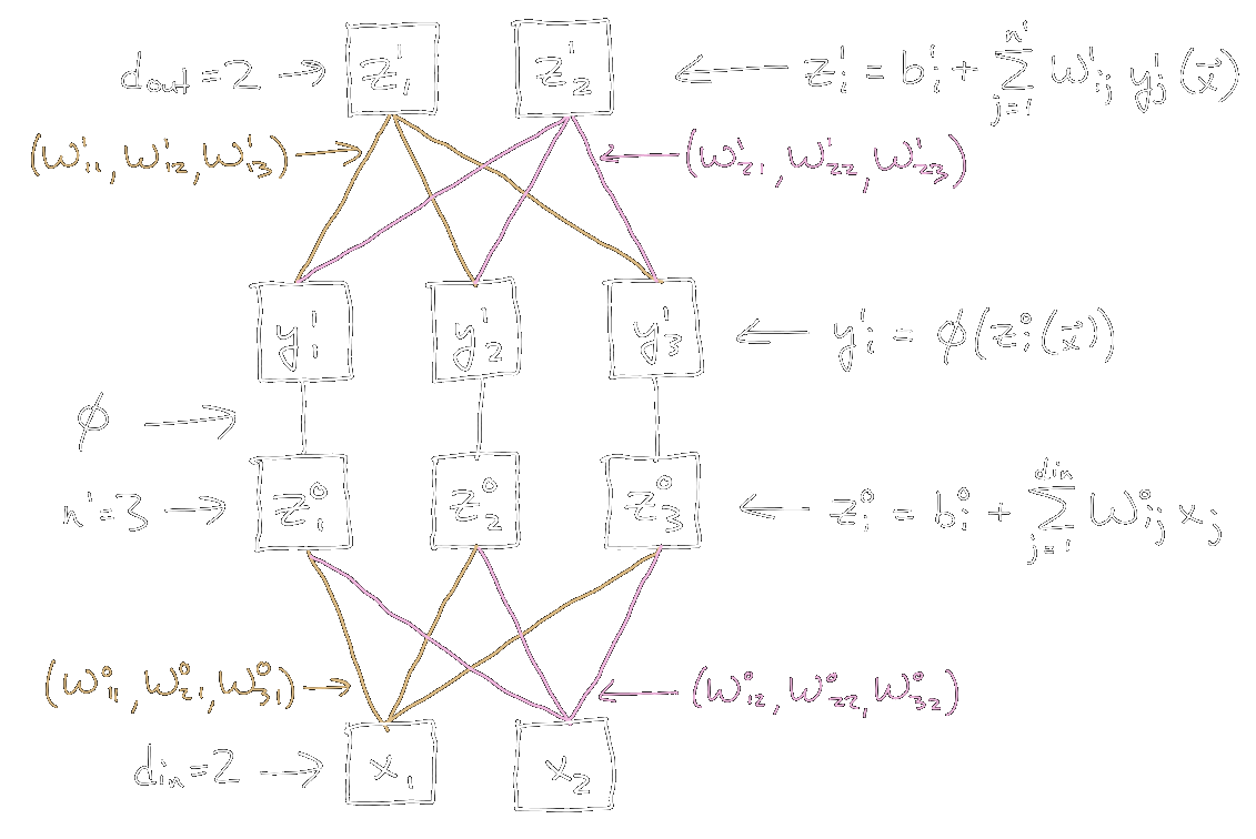 |
|---|
| Figure 2: Single hidden layer network, with \(d_{\textrm{in}} = 2\), \(d_{\textrm{out}} = 2\), \(n^1 = 3\). For simplicity, the biases \(b_i^0\) and \(b_i^1\) are not drawn. |
Next, recall that a Gaussian process is defined by its mean, \(\mu(\vec x)\), and
covariance, \(C(\vec x, \vec x')\), given two values of the input vector \(\vec x\) and
\(\vec x'\). We say that \(a(\vec x)\) is drawn from a Gaussian process, \(a(\vec x)
\sim \mathcal{GP}(\vec \mu, \mathbf{C})\), if any finite number \(p\) of draws
\(\{a(\vec x^{(1)}), \dots, a(\vec x^{(p)}) \}\) follows a multivariate normal
distribution \(\mathcal{N}(\vec \mu, \mathbf{C})\), with
Looking at the preactivations going into the hidden layer, we see that for each \(i\), \(z_i^0 | \vec x\) is a Gaussian process: \(z_i^0\) is a linear combination of the \(b_i^0\) weight and the \(W_{ij}^0\) weights, and each of these weights is an independent Gaussian variable, so \(z_i^0\) will also be Gaussian. The linear combination coefficients are the components of \(\vec x\).
We can calculate the mean and covariance functions for this process as
\[\begin{align} \mu(\vec x) &= \mathbb{E}[z_i^0(\vec x)] = \mathbb{E}[b_i^0] + \sum_{j=1}^{d_{\textrm{in}}} \mathbb{E}[W_{ij}^0] x_j = 0\nonumber\\ C^0(\vec x, \vec x') &= \mathbb{E}[z_i^0(\vec x) z_i^0(\vec x')]\nonumber\\ &= \mathbb{E} \left[ \left(b_i^0 + \sum_{k=1}^{d_{\textrm{in}}} W_{ik}^0 x_k \right) \left(b_i^0 + \sum_{m=1}^{d_{\textrm{in}}} W_{im}^0 x_m' \right) \right]\nonumber\\ &= \mathbb{E}[b_i^0 b_i^0] + \mathbb{E}\left[ b_i^0 \sum_{m=1}^{d_{\textrm{in}}} W_{im}^0 x_m' \right] + \mathbb{E}\left[ b_i^0 \sum_{k=1}^{d_{\textrm{in}}} W_{ik}^0 x_k\right]\nonumber\\ &\quad\quad\quad\quad\,\,+ \mathbb{E}\left[\left( \sum_{k=1}^{d_{\textrm{in}}} W_{ik}^0 x_k \right) \left( \sum_{m=1}^{d_{\textrm{in}}} W_{im}^0 x_m' \right)\right]\nonumber\\ &= \sigma_b^2 + 0 + 0 + \delta_{km} \frac{\sigma_w^2}{d_{\textrm{in}}} \left(\sum_{k=1}^{d_{\textrm{in}}} x_k \right) \left(\sum_{m=1}^{d_{\textrm{in}}} x_m' \right)\nonumber\\ &= \sigma_b^2 + \frac{\sigma_w^2}{d_{\textrm{in}}} \sum_{k=1}^{d_{\textrm{in}}} x_k x_k'\nonumber\\ &= \sigma_b^2 + \sigma_w^2 \frac{\vec x \cdot \vec x'}{d_{\textrm{in}}}\nonumber\\ &= \sigma_b^2 + \sigma_w^2 K^0(\vec x, \vec x') \end{align}\]where the cross terms in the third line vanish because \(\mathbb{E}[b_i^0 W_{jk}^0] = 0\), and we have defined \(K^0(\vec x, \vec x') \equiv \vec x \cdot \vec x' / d_{\textrm{in}}\) in the last line.
If we look at the covariance between two different preactivation components, \(z_i^0\) and \(z_j^0\), for \(i \neq j\), we see that they are independent since
\[\begin{align} \mathbb{E}[z_i^0(\vec x) z_j^0(\vec x')] &= \mathbb{E}[b_i^0 b_j^0] + 0 + 0 + \mathbb{E}\left[\left(\sum_{k=1}^{d_{\textrm{in}}} W_{ik}^0 x_k \right) \left( \sum_{m=1}^{d_{\textrm{in}}} W_{jm}^0 x_m' \right)\right]\nonumber\\ &= \delta_{ij} \sigma_b^2 + \delta_{ij} \delta_{km} \frac{\sigma_w^2}{d_{\textrm{in}}} \left(\sum_{k=1}^{d_{\textrm{in}}} x_k \right) \left(\sum_{m=1}^{d_{\textrm{in}}} x_m' \right)\nonumber\\ &= 0,\quad i \neq j \end{align}\]Thus every component of the preactivation computes an independent sample of the same Gaussian process, \(\mathcal{GP}(0, C^0(\vec x, \vec x'))\).
Next, we go up one layer and look at the network outputs \(z_i^1(\vec x)\). Following the same line of reasoning as for the \(z_i^0(\vec x)\), we see that for each \(i\), \(z_i^1 | \vec y^1\) is a Gaussian process. The mean and covariance functions here are
\[\begin{align} \mu(\vec x) &= \mathbb{E}[z_i^1(\vec x)] = \mathbb{E}[b_i^1] + \sum_{j=1}^{n^1} \mathbb{E}[W_{ij}^1] y_j^1(\vec x) = 0\nonumber\\ C^1(\vec x, \vec x') &= \mathbb{E}[z_i^1(\vec x) z_i^1(\vec x')]\nonumber\\ &= \mathbb{E} \left[ \left(b_i^1 + \sum_{k=1}^{n^1} W_{ik}^1 y_k^1(\vec x) \right) \left(b_i^1 + \sum_{m=1}^{n^1} W_{im}^1 y_m^1(\vec x') \right) \right]\nonumber\\ &= \mathbb{E}[b_i^1 b_i^1] + \mathbb{E}\left[ b_i^1 \sum_{m=1}^{n^1} W_{im}^1 y_m^1(\vec x') \right] + \mathbb{E}\left[ b_i^1 \sum_{k=1}^{n^1} W_{ik}^1 y_k^1(\vec x) \right]\nonumber\\ &\quad\quad\quad\quad\,\, + \mathbb{E}\left[\left( \sum_{k=1}^{n^1} W_{ik}^1 y_k^1(\vec x) \right) \left( \sum_{m=1}^{n^1} W_{im}^1 y_m^1(\vec x') \right)\right]\nonumber\\ &= \sigma_b^2 + 0 + 0 + \delta_{km} \frac{\sigma_w^2}{n^1} \left(\sum_{k=1}^{n^1} y_k^1(\vec x) \right) \left(\sum_{m=1}^{n^1} y_m^1(\vec x') \right)\nonumber\\ &= \sigma_b^2 + \sigma_w^2 \left( \frac{1}{n^1} \sum_{k=1}^{n^1} y_k^1(\vec x) y_k^1(\vec x') \right)\nonumber\\ &= \sigma_b^2 + \sigma_w^2 K^1(\vec x, \vec x') \end{align}\]where we have defined the kernel \(K^1(\vec x,\vec x') \equiv \frac{1}{n^1} \sum_{k=1}^{n^1} y_k^1(\vec x) y_k^1(\vec x')\) in the last line. The cross terms in the third line vanish because \(\mathbb{E}[b_i^1 W_{jk}^1] = 0\). The final terms in the third and fourth line are equal because \(\mathbb{E}[W_{ik}^1 y_k^1(\vec x)] = 0\), which follows from the fact that \(y_k^1(\vec x)\) depends only on \(W_{ik}^0\) and \(b_i^0\), both of which are independent of \(W_{ik}^1\).
Again, following the same line of reasoning as for the \(z_i^0(\vec x)\), if we look at the covariance between two different components of the output, \(z_i^1\) and \(z_j^1\), for \(i \neq j\), we see that they are independent, since
\[\begin{align} \mathbb{E}[z_i^1(\vec x) z_j^1(\vec x')] &= \mathbb{E}[b_i^1 b_j^1] + 0 + 0 + \mathbb{E}\left[\left(\sum_{k=1}^{d_{\textrm{in}}} W_{ik}^0 y_m^1(\vec x') \right) \left( \sum_{m=1}^{d_{\textrm{in}}} W_{jm}^0 y_m^1(\vec x') \right)\right]\nonumber\\ &= \delta_{ij} \sigma_b^2 + \delta_{ij} \delta_{km} \frac{\sigma_w^2}{d_{\textrm{in}}} \left(\sum_{k=1}^{d_{\textrm{in}}} y_k^1(\vec x) \right) \left(\sum_{m=1}^{d_{\textrm{in}}} y_m^1(\vec x') \right)\nonumber\\ &= 0,\quad i \neq j \end{align}\]so that every component of the output computes an independent sample of the Gaussian process \(\mathcal{GP}(0, C^1(\vec x, \vec x'))\). The multiple outputs of the network are therefore redundant: there is no difference between a network with \(d_{\textrm{out}}\) outputs, and \(d_{\textrm{out}}\) copies of an equivalent network but with only one output.
Substituting \(\phi\) back into the definition of \(y_i^1\), we have
\begin{equation} K^1(\vec x,\vec x’) = \frac{1}{n^1} \sum_{k=1}^{n^1} \phi(z_k^0(\vec x)) \phi(z_k^0(\vec x’)). \end{equation}
Now since each term in this sum depends on an independent sample \(\{z_k^0(\vec x), z_k^0(\vec x')\}\) from the Gaussian process \(\mathcal{GP}(0, C^0(\vec x, \vec x'))\), in the limit as \(n^1 \to \infty\) we can use the law of large numbers to obtain
\[\begin{equation} \lim_{n^1 \to \infty} K^1(\vec x,\vec x') = \!\!\!\! \iint\limits_{z,z' = -\infty}^{\infty}\!\!\!\! dz dz' \phi(z) \phi(z') \mathcal{N}\left(z, z'; 0, \sigma_b^2 \mathbf{I}_2 + \sigma_w^2 \left[\begin{matrix} K^0(\vec x, \vec x) & K^0(\vec x, \vec x')\\ K^0(\vec x', \vec x) & K^0(\vec x', \vec x') \end{matrix} \right] \right) \end{equation}\]where \(\mathbf{I}_2\) is the \(2 \times 2\) identity matrix. This integral can be evaluated in closed form for certain choices of \(\phi\) (see Cho & Saul (2009)), but in general it must be computed numerically. An efficient algorithm for this computation was provided by Lee et al. (2017).
We now have a form for the kernel \(K^1(\vec x,\vec x')\), computed deterministically in terms of the kernel of the previous layer, \(K^0(\vec x,\vec x')\). This gives us the final, output Gaussian process for the entire network via \(C^1(\vec x, \vec x') = \sigma_b^2 + \sigma_w^2 K^1(\vec x, \vec x')\). In order to use the Gaussian process to make a test prediction, we must:
-
Calculate the kernel \(K^0(\vec x,\vec x')\) for all pairs taken from the set of training and test inputs. e.g. for \(p\) training inputs and test input \(\vec x^*\), both \(\vec x\) and \(\vec x'\) range over \(\{ \vec x^{(1)}, \dots, \vec x^{(p)}, \vec{x}^* \}\), so we need to calculate \((p+1)(p+2)/2\) quantities (as the kernel matrix is symmetric).
-
Calculate the kernel \(K^1(\vec x,\vec x')\) for all the above pairs (in terms of \(K^0(\vec x,\vec x')\)), again yielding \((p+1)(p+2)/2\) quantities. The covariance matrix for the output Gaussian process then has elements \(C^1(\vec x, \vec x') = \sigma_b^2 + \sigma_w^2 K^1(\vec x, \vec x')\), where \(\vec x, \vec x' \in \{ \vec x^{(1)}, \dots, \vec x^{(p)}, \vec{x}^* \}\)
-
Use the output Gaussian process in the standard fashion to make a prediction for the test input, by marginalizing over the training input variables in the multivariate Gaussian defined by
MULTIPLE LAYERS
The generalization to an arbitrary number \(L \geq 2\) of hidden layers is straightforward, as all of the relevant calculations were done in the single-hidden-layer case.
The only additional step is to write the general expression for the \(\ell\)th layer’s outputs \(z_i^\ell(\vec x)\) in terms of the preactivations \(z_i^{\ell-1}(\vec x)\) of the previous layer:
\[\begin{equation} z_i^\ell(\vec x) = b_i^\ell + \sum_{j=1}^{n^\ell} W_{ij}^\ell \phi(z_j^{\ell-1}(\vec x))\quad \begin{cases} 1 \leq i \leq n^{\ell+1}, &\text{for $1 \leq \ell < L$}\\ 1 \leq i \leq d_{\textrm{out}}, &\text{for $\ell = L$} \end{cases} \end{equation}\]where the \(W_{ij}^\ell \sim \mathcal{N}(0, \sigma_w^2 / n^\ell)\) and \(b_i^\ell \sim \mathcal{N}(0, \sigma_b^2)\) are all i.i.d. for each layer \(\ell\). The weight orthogonality relations for each layer are
\[\begin{equation} \mathbb{E}[W_{ij}^\ell W_{km}^\ell] = \delta_{ik} \delta_{jm} \frac{\sigma_w^2}{n^\ell}, \quad \mathbb{E}[b_i^\ell b_j^\ell] = \delta_{ij} \sigma_b^2, \quad \mathbb{E}[b_i^\ell W_{jk}^\ell] = 0, \qquad 1 \leq \ell \leq L. \end{equation}\]Similar to the relation between \(K^1(\vec x,\vec x')\) and \(K^0(\vec x,\vec x')\), in the limit as \(n^\ell \to \infty\) the expression for the kernel at layer \(\ell\) can be written as a deterministic function of the kernel at layer \(\ell-1\):
\[\begin{equation} K^\ell(\vec x,\vec x') = \frac{1}{n^\ell} \sum_{k=1}^{n^\ell} \phi(z_k^{\ell-1}(\vec x)) \phi(z_k^{\ell-1}(\vec x')), \end{equation}\] \[\begin{equation} \lim_{n^\ell \to \infty} K^\ell(\vec x,\vec x') = \!\!\!\! \iint\limits_{z,z' = -\infty}^{\infty}\!\!\!\! dz dz' \phi(z) \phi(z') \mathcal{N}\left(z, z'; 0, \sigma_b^2 \mathbf{I}_2 + \sigma_w^2 \left[\begin{matrix} K^{\ell-1}(\vec x, \vec x) & K^{\ell-1}(\vec x, \vec x')\\ K^{\ell-1}(\vec x', \vec x) & K^{\ell-1}(\vec x', \vec x') \end{matrix} \right] \right) \end{equation}\]which applies for all \(1 \leq \ell \leq L\).
To calculate the covariance matrix \(C^L(\vec x, \vec x')\) for the final ouput layer, we first repeat the initial step from the single-hidden-layer case to calculate \(K^0(\vec x, \vec x')\) for all \(\vec x, \vec x' \in \{ \vec x^{(1)}, \dots, \vec x^{(p)}, \vec{x}^* \}\). Next, for each \(\ell \in (1, \dots, L)\), in sequence, we calculate \(K^\ell(\vec x, \vec x')\) in terms of \(K^{\ell-1}(\vec x, \vec x')\), for all \(\vec x, \vec x' \in \{ \vec x^{(1)}, \dots, \vec x^{(p)}, \vec{x}^* \}\). Finally, given the final \(C^L(\vec x, \vec x')\), we can make predictions for the test input \(\vec x^*\) in the standard fashion for Gaussian processes.
Discussion and Conclusions
We’ve shown how to compute a Gaussian process that is equivalent to an \(L\)-layer neural network at initialization, in the limit as the hidden layer widths become infinite. This gives us an analytic handle on the problem, and allows us to do Bayesian inference for regression by applying matrix computations, obtaining predictions and uncertainty estimates for the network, without doing any SGD training.
The form of the Gaussian process covariance matrix, \(C^L(x, x')\), depends only on a few hyperparameters: the network depth \(L\), the choice of \(\phi\), and the choice of \(\sigma_w^2\) and \(\sigma_b^2\). One interesting question is how the choice of \(\sigma_w^2\) and \(\sigma_b^2\) affects the performance of the Gaussian process. The answer comes from a fascinating related line of research into deep signal propagation, starting with the papers Poole et al. (2016) and Schoenholz et al. (2017), which I’ll cover in a future blog post.
In the process of understanding the computations involved in the NNGP, I benefited greatly from Jascha Sohl-Dickstein’s talk “Understanding overparameterized neural networks” at the ICML 2019 workshop: Theoretical Physics for Deep Learning.
Thanks to Brandon DiNunno for helpful comments and suggestions on this post.