Introduction
In a previous post, I talked about neural network Gaussian processes (NNGPs), and how they let us do exact Bayesian inference for neural networks at initialization, in the limit of large layer width, via straightforward matrix computations. This is great, but there are two big open questions:
- Can we use a similar technique to describe the network during training, rather than just at initialization?
- Can we use this formalism to describe networks with finite layer widths?
The first question was addressed by Jacot et al. (2018), with the introduction of the Neural Tangent Kernel. They showed that under certain conditions, the output \(f(x)\) of a wide multilayer neural network behaves as
\[\begin{align} \frac{d f(x)}{d t} &=-\sum_{(x',y') \in D_{\textrm{tr}}} \sum_\mu \frac{\partial f(x)}{\partial\theta^\mu} \frac{\partial f(x')}{\partial \theta^\mu} \frac{\partial \ell(x',y')}{\partial f}\nonumber\\ &=-\sum_{(x',y') \in D_{\textrm{tr}}}\Theta(x,x')\frac{\partial \ell(x',y')}{\partial f} \end{align}\]during training. Here \(D_{\textrm{tr}}\) is the training set, \((x', y')\) is a specific training input and target value pair, the \(\theta^\mu\) are the weights of the neural network, \(\ell(x', y')\) is the single sample loss, such that the total loss \(L = \sum_{(x',y') \in D_{\textrm{tr}}} \ell(x',y')\), and we have defined \(\Theta(x, x') = \sum_\mu \left( \partial f(x) / \partial \theta^\mu \right) \left( \partial f(x') / \partial \theta^\mu \right)\) as the Neural Tangent Kernel (NTK). If we use the mean squared error (MSE) for our loss, we have
\begin{equation} \frac{d f(x)}{d t} = -\sum_{(x’,y’) \in D_{\textrm{tr}}} \Theta(x,x’) (f(x’) - y’) \end{equation}
I won’t go through the details of the NTK here, but a good overview can be found in these two blog posts. One result of Jacot et al. (2018) is that the NTK is constant during training in the large width limit, which means we can just use its value at initialization.
The NTK lets us describe the evolution of the network function \(f(x)\) in terms of the training set inputs, without having to run gradient descent. However if we want to describe the evolution of a finite width network, the NTK is no longer constant during training, and we need a way to compute corrections due to the finite width. This brings us to our second question, which is the main focus of this post.
A method for computing finite width corrections was introduced in Dyer and Gur-Ari (2019). The authors use a tool known to physicists as Feynman diagrams to develop a technique for simple calculation of the large-\(\mathit{n}\) scaling behavior of a wide class of network quantities, including the network function, the NTK, and their time derivatives. Here, \(n\) is the width of each hidden layer. Although the technique only specifies how these quantities scale with \(n\), rather than their exact value, it is far quicker than performing the full calculation.
After introducing some notation, we’ll talk about the quantities we want to compute, called correlation functions. We’ll warm up by computing some simple cases for a network with a single hidden layer and linear activation. Next we’ll introduce Feynman diagrams, which help keep track of the terms in correlation functions. We’ll then cover more general correlation functions and multilayer networks. Finally, we’ll show how to use our results to compute finite width corrections to the network function and NTK during training.
Notation
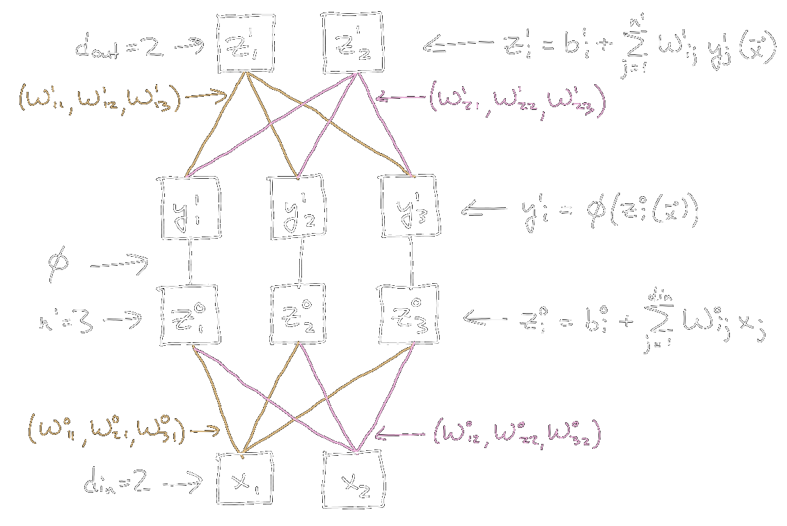
We follow the conventions in Dyer and Gur-Ari (2019), with some modifications for simplicity. We consider a fully connected neural network with \(d\) hidden layers, a one-dimensional input \(x \in \mathbb{R}\), and a one-dimensional output given by the network function \(f(x) \in \mathbb{R}\). Multiple values of the input \(x\) are distinguished with subscripts, e.g. a set of \(p\) training examples is \(\{x_1, \dots, x_p\}\). Weights from the input to the first hidden layer are \(U \in \mathbb{R}^n\), and those from the final hidden layer to the output are \(V \in \mathbb{R}^n\). For networks with more than one hidden layer, the weights between layer \(l\) and \(l+1\) are \(W^{(l)} \in \mathbb{R}^{n \times n}\). The network activation function is \(\sigma\).
With this notation, the network function is
\begin{equation} f(x) = n^{-d/2} V^T \sigma\Big(W^{(d-1)}\dots\sigma\big(W^{(1)} \sigma(Ux)\big)\Big) \end{equation}
with \(V\) transposed to make the matrix multiplication work out. The components of \(U, V\) and the \(W^{(l)}\) are drawn i.i.d. from a normal distribution \(\mathcal{N}(0, 1)\) at initialization, and we collect them into a vector \(\theta\) with components \(\theta^\mu\).
We limit our calculations to \(d \leq 2\) hidden layers, in which case we write \(W\) instead of \(W^{(1)}\). We also adopt Einstein summation convention, where vectors have (column) components \(A^i\), transpose vectors have (row) components \(A_i\), matrices have components \(W^i_j\), and summation is implied over repeated upper and lower indices.
For example, the network function for a two layer linear network (\(\sigma = 1\)) is
\begin{equation} f(x)=n^{-1} V^T W U x = n^{-1} V_i W^i_j U^j x \end{equation}
with an implied summation over \(i\) and \(j\).
The covariances between the weights are given by the weight orthogonality relations, which read
\[\begin{equation} \mathbb{E}_\theta \left[ U^i U^j \right] = \delta^{ij},\quad \mathbb{E}_\theta \left[ V_i V_j \right] = \delta_{ij},\quad \mathbb{E}_\theta \left[ W^i_j W^k_m \right] = \delta^{ik} \delta_{jm} \end{equation}\]and vanish between all remaining components. The expression for \(W\) applies separately for each layer, and vanishes between components in different layers. The Kronecker delta \(\delta^{ij} = \delta_{ij}\) equals 1 when \(i = j\) and 0 otherwise.
We will often use the fact that the trace of the product of any number of Kronecker deltas equals \(n\), e.g.
\begin{equation} \delta_{ij} \delta^{ij} = \delta_{ij} \delta^{jk} \delta_{km} \delta^{mi} = n, \end{equation}
which follows since the Kronecker delta is just the \(n \times n\) identity matrix. We sometimes use angle brackets to denote an expectation over the network weights \(\theta\), e.g.
\begin{equation} \langle U^i U^j \rangle \equiv \mathbb{E}_\theta \left[ U^i U^j \right] \end{equation}
For ease of reference, all definitions, conjectures, theorems, and lemmas taken from Dyer and Gur-Ari (2019) are given the same numbers as in the paper.
Correlation Functions and Isserlis’ Theorem
We are interested in calculating correlation functions, which are ensemble averages of the network function \(f(x)\), its products, and (eventually) its derivatives, with respect to the network weights \(\theta\), evaluated on arbitrary inputs. For example, in the NNGP post we calculated the covariance function \(C^1(x_1, x_2)\) for an wide, \(n\)-unit single layer network,
\[\begin{equation} C^1(x_1, x_2) = \mathbb{E}_\theta \left[ f(x_1) f(x_2) \right]. \end{equation}\]If we consider a single layer linear network, we have
\[\begin{equation} \mathbb{E}_\theta \left[ f(x_1) f(x_2) \right] = n^{-1} \mathbb{E}_\theta \left[ V_i U^i x_1 V_j U^j x_2 \right] = n^{-1} \mathbb{E}_\theta \left[ V_i U^i V_j U^j \right] x_1 x_2. \end{equation}\]The \(U^i\) and \(V_j\) are components of \(\theta\), which is a zero-mean multivariate Gaussian distribution, so we can evaluate \(\mathbb{E}_\theta \left[ V_i U^i V_j U^j \right]\) by applying Isserlis’ theorem, which expresses the higher-order moments of a multivariate Gaussian in terms of its covariance matrix.
Theorem (Isserlis) Let \(\left( \theta^1, \dots, \theta^p \right)\) be a zero-mean multivariate Gaussian random vector, then for \(k\) a positive integer
\[\begin{equation} \mathbb{E}_\theta\left[\theta^1, \dots, \theta^{k}\right]= \begin{cases} \sum_{p \in P^2_{k}}\prod_{i \in \{i,j\}}\mathbb{E}_\theta\left[\theta^i \theta^j\right], &\text{for k even};\\ 0, &\text{for k odd.} \end{cases} \end{equation}\]where the sum is over all distinct ways of partitioning \(\{1, \dots, k \}\) into pairs \(\{i,j\}\), and the product is over the pairs contained in \(p\).
For example, Isserlis’ theorem for four variables is
\[\begin{equation} \mathbb{E}_\theta \left[ \theta^1 \theta^2 \theta^3 \theta^4 \right] = % \frac{1}{2!} \mathbb{E}_\theta \left[ \theta^1 \theta^2 \right] \mathbb{E}_\theta \left[ \theta^3 \theta^4 \right] + \mathbb{E}_\theta \left[ \theta^1 \theta^3 \right] \mathbb{E}_\theta \left[ \theta^2 \theta^4 \right] + \mathbb{E}_\theta \left[ \theta^1 \theta^4 \right] \mathbb{E}_\theta \left[ \theta^2 \theta^3 \right]. \end{equation}\]Applying this to our single layer linear network, with \(\left( \theta^1, \theta^2, \theta^3, \theta^4 \right) = \left( V_i, U^i, V_j, U^j \right)\), we get
\[\begin{equation} \begin{split} \mathbb{E}_\theta&\left[ f(x_1) f(x_2) \right] = n^{-1} \mathbb{E}_\theta \left[ V_i U^i V_j U^j \right] x_1 x_2\\ &= n^{-1}\left( \langle V_i U^i \rangle \langle V_j U^j \rangle + \langle V_i V_j \rangle \langle U^i U^j \rangle + \langle V_i U^j \rangle \langle U^i V_j \rangle \right) x_1 x_2 \\ &= n^{-1} \langle V_i V_j \rangle \langle U^i U^j \rangle x_1 x_2 \\ &= n^{-1} \left( \delta_{ij} \delta^{ij} \right) x_1 x_2 \\ &= x_1 x_2 \sim \mathcal{O}(n^0) \end{split} \label{eq:2pt_1hl} \end{equation}\]where the second and third lines follow from the weight orthogonality relations, and the final expression follows from the rule for the trace of the product of Kronecker deltas. This expression scales as \(\mathcal{O}(n^0)\), or constant scaling.
The next level up in complexity is the four-point correlation function, which has nine terms.
\[\begin{equation} \begin{split} \mathbb{E}_\theta &\left[ f(x_1) f(x_2) f(x_3) f(x_4) \right] = n^{-2}\mathbb{E}_\theta \left[ V_i U^i V_j U^j V_k U^k V_m U^m \right] x_1 x_2 x_3 x_4\\ &= n^{-2}\left( \langle V_i V_j \rangle \langle V_k V_m \rangle + \langle V_i V_k \rangle \langle V_j V_m \rangle + \langle V_i V_m \rangle \langle V_j V_k \rangle \right) \times\\ &\qquad\ \ \, \left(\langle U^i U^j \rangle \langle U^k U^m \rangle + \langle U^i U^k \rangle \langle U^j U^m \rangle + \langle U^i U^m \rangle \langle U^j U^k \rangle \right) x_1 x_2 x_3 x_4\\ &= n^{-2} \left( \delta_{ij}\delta_{km} + \delta_{ik}\delta_{jm} + \delta_{im}\delta_{jk} \right) \left( \delta^{ij}\delta^{km} + \delta^{ik}\delta^{jm} + \delta^{im}\delta^{jk} \right) x_1 x_2 x_3 x_4\\ &= n^{-2} \left[ 3 \left( \delta_{ij} \delta^{ij} \right) \left( \delta_{km} \delta^{km} \right) + 6 \left( \delta_{ij} \delta^{jk} \delta_{km} \delta^{mi} \right) \right] x_1 x_2 x_3 x_4\\ &= \left( 3 + 6 n^{-1} \right) x_1 x_2 x_3 x_4 \sim \mathcal{O}(n^0) \end{split} \label{eq:4pt_1hl} \end{equation}\]The second line follows from Isserlis’ theorem with \(k=8\) and the weight orthogonality relations, which are also used in the third line. The fourth line collects terms with similar structure, by relabeling Kronecker delta indices and using the symmetry of \(\delta_{ij} = \delta_{ji}\). The last line follows from the rule for the trace of the product of Kronecker deltas. This correlation function also scales as \(\mathcal{O}(n^0)\), but has an additional \(\mathcal{O}(n^{-1})\) correction.
Feynman Diagrams as a Calculational Shortcut
Keeping track of the Kronecker delta sums becomes unwieldy as correlation functions get more complicated. This annoyed Feynman way back in the 1940s when he was doing similar calculations in quantum field theory, so he invented a diagrammatic technique to help. In our situation, every correlation function \(C\) has an associated set of graphs, \(\Gamma(C)\), called Feynman diagrams, defined as
Definition 2. Let \(C(x_1, \dots, x_m)\) be a correlation function for a network with \(d\) hidden layers. \(\Gamma(C)\) is the set of all graphs that have the following properties.
- There are \(m\) vertices \(v_1, \dots, v_m\), each of degree (number of edges) \(d+1\).
- Each edge has a type \(t \in \{ U, W^{(1)}, \dots, W^{(d-1)}, V \}\). Every vertex has one edge of each type.
The graphs in \(\Gamma(C)\) are called the Feynman diagrams of \(C\).
Let’s walk through this definition for the two single layer correlation functions we’ve computed so far.
For \(\mathbb{E}_\theta \left[ f(x_1) f(x_2) \right]\), each diagram has two vertices of degree two, while each edge has type \(U\) or \(V\). There is only one diagram, shown in Figure 1:
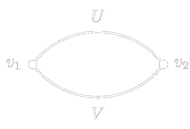
Figure 1: The Feynman diagram for the two-point function of a single layer network.
We can compute how a diagram scales with \(n\) by using the Feynman rules: 1) each
vertex contributes a factor of \(n^{-1/2}\), and 2) each loop contributes a factor of
\(n\). The above diagram has two vertices and one loop, so it scales as
\(\mathcal{O}(n^0)\), agreeing with the result of Eq. \eqref{eq:2pt_1hl}.
To motivate the rules we inspect the second-to-last line of that calculation, \(n^{-1} \left( \delta_{ij} \delta^{ij} \right) x_1 x_2\). The \(n^{-1}\) factor comes from the two \(n^{-1/2}\) terms in the network function definitions, which motivates the first rule. The \(\delta_{ij}\) and \(\delta^{ij}\) are from \(\mathbb{E}_\theta \left[ V_i V_j \right]\) and \(\mathbb{E}_\theta \left[ U^i U^j \right]\), which correspond to edges, and the \(\delta_{ij} \delta^{ij}\) sum corresponds to the loop, giving a factor of \(n\) and motivating the second rule.
For \(\mathbb{E}_\theta \left[ f(x_1) f(x_2) f(x_3) f(x_4) \right]\), each diagram has four vertices of degree two, with each edge of type \(U\) or \(V\). There are nine diagrams, shown in Figure 2, corresponding to the nine terms that come from expanding out \(\left( \delta_{ij}\delta_{km} + \delta_{ik}\delta_{jm} + \delta_{im}\delta_{jk} \right) \left( \delta^{ij}\delta^{km} + \delta^{ik}\delta^{jm} + \delta^{im}\delta^{jk} \right)\) in Eq. \eqref{eq:4pt_1hl}.
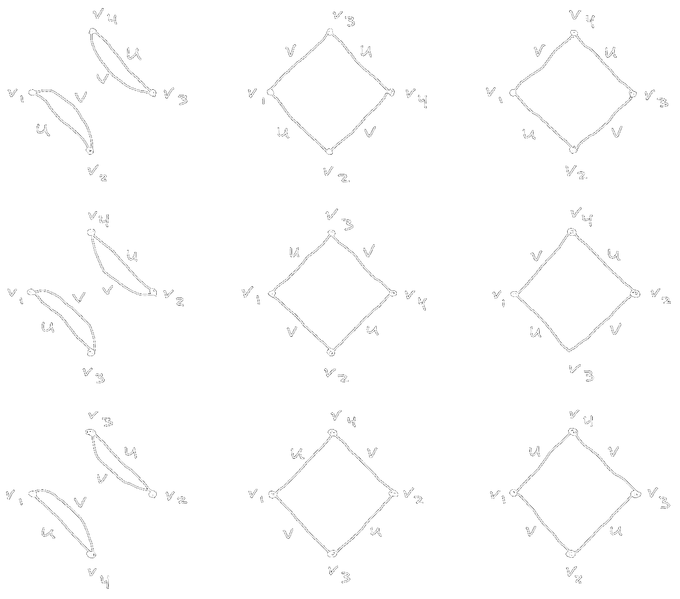
Figure 2: The nine diagrams for the four-point function of a single layer network. Vertices have been rearranged to make diagrams of the same topology look similar.
The Feynman rules only care about the topology of a diagram — the number of
vertices and loops — and not how the edges are connected within a given topology. The
nine diagrams in Figure 2 have two topological types. The first has two disconnected loops
and corresponds to the \(n^{-2}\, 3 \left( \delta_{ij} \delta^{ij} \right) \left(
\delta_{km} \delta^{km} \right)\) term in Eq. \eqref{eq:4pt_1hl}, which scales as
\(\mathcal{O}(n^0)\). The second has a single loop and corresponds to the \(n^{-2}\, 6
\left( \delta_{ij} \delta^{jk} \delta_{km} \delta^{mi} \right)\) term, scaling as
\(\mathcal{O}(n^{-1})\). The factors of 3 and 6 come from the number of diagrams of each
type. The entire correlation function thus scales as \(\mathcal{O}(n^0)\), implying that
the diagram with the largest number of loops determines the scaling. This is stated as a
theorem:
Theorem 3. Let \(C(x_1, \dots, x_m)\) be a correlation function with one hidden layer and linear activation. Let \(\gamma\) be a diagram in \(\Gamma(C)\). Then \(C = \mathcal{O}(n^s)\) where \(s = \mathrm{max}_{\gamma \in \Gamma(C)} \left( l_\gamma - m/2 \right)\), and \(l_\gamma\) is the number of loops in \(\gamma\).
For correlation functions more complicated than the two we have worked through, it is much easier to determine the possible diagram topologies than to expand out all the terms and keep track of the \(\delta_{ij}\) sums. In fact, for an \(m\)-point correlation function the scaling behavior will always be dominated by the diagram with \(m/2\) disconnected bubbles.
Multilayer Networks
The analysis changes for networks with multiple layers, so let’s look at a two layer network. The two-point correlation function is
\[\begin{equation} \label{eq:2pt_2hl} \begin{split} \mathbb{E}_\theta &\left[ f(x_1) f(x_2) \right] = n^{-2}\mathbb{E}_\theta \left[ V_i W^i_j U^j V_k W^k_m U^m \right] x_1 x_2\\ &= n^{-2}\left( \langle V_i V_k \rangle \langle U^j U^m \rangle \langle W^i_j W^k_m \rangle \right) x_1 x_2\\ &= n^{-2}\left( \delta_{ik} \delta^{ik} \delta_{jm} \delta^{jm} \right) x_1 x_2\\ &= x_1 x_2 \sim \mathcal{O}(n^0) \end{split} \end{equation}\]There is only one diagram, shown in Figure 3. Each vertex has degree three, and there are now three types of edges, \(U, W, V\).
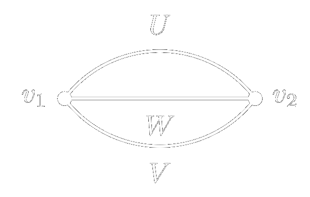
Figure 3: The diagram for the two-point function of a two layer network.
However, the number of loops in this diagram is ambiguous. The solution to this problem
is due to ‘t Hooft
(1973):
we transform each diagram \(\gamma\) into an equivalent double-line diagram
\(\textrm{DL}(\gamma)\), as follows.
For a network with \(d\) hidden layers,
- Each vertex \(v_i\) in \(\gamma\) is mapped to \(d\) vertices \(v^{(1)}_i,\dots,v^{(d)}_i\) in \(\textrm{DL}(\gamma)\).
- Each edge \((v_i,v_j)\) in \(\gamma\) of type \(W^{(l)}\) is mapped to two edges \((v^{(l)}_i,v^{(l)}_j)\), \((v^{(l+1)}_i,v^{(l+1)}_j)\).
- Each edge \((v_i,v_j)\) in \(\gamma\) of type \(U\) is mapped to a single edge \((v^{(1)}_i,v^{(1)}_j)\).
- Each edge \((v_i,v_j)\) in \(\gamma\) of type \(V\) is mapped to a single edge \((v^{(d)}_i,v^{(d)}_j)\).
We have \(d=2\), so each vertex is replaced by two vertices, and the \(W\) edge is replaced by two edges. See Figure 4.
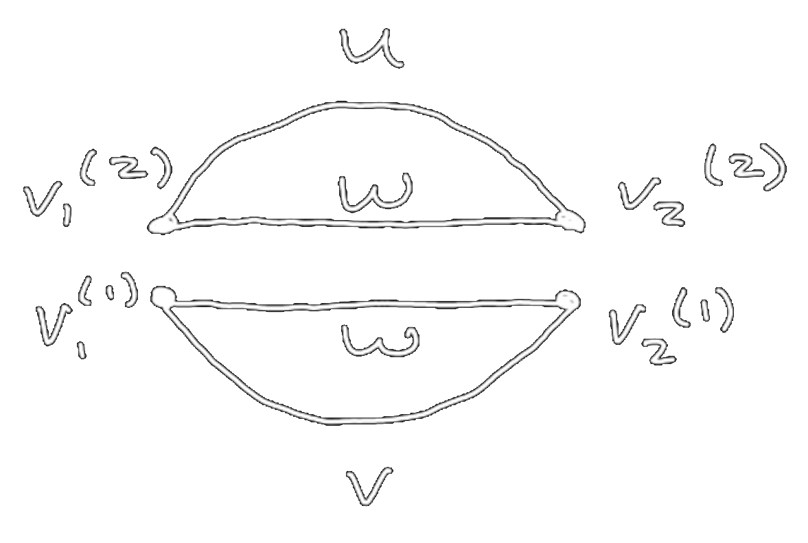
Figure 4: The double-line diagram for the two-point function of a two layer network.
The ambiguity in the number of loops has been resolved — the double-line graph clearly
has two loops. To calculate the scaling, we use the Feynman rules, but applied to the
double-line graph. The four vertices contribute \(n^{-2}\), and the two loops contribute
\(n^{2}\), yielding the expected \(\mathcal{O}(n^0)\) scaling.
Correlation Functions with Derivatives
More generally, we want to calculate correlation functions of products of derivative tensors of the network function \(f(x)\), where the rank-\(k\) derivative tensor is \(T_{\mu_1 \dots \mu_k}(x) \equiv \partial^k f(x)\,/\, \partial \theta^{\mu_1} \cdots \partial \theta^{\mu_k}\), and the rank-0 derivative tensor is just \(f(x)\) itself. For example, the NTK ensemble average is
\[\begin{equation} \label{eq:tensor1} \mathbb{E}_\theta\left[ \Theta \left( x_1, x_2 \right) \right] = \sum_\mu \mathbb{E}_\theta\left[ \frac{\partial f(x_1)}{\partial \theta^\mu} \frac{\partial f(x_2)}{\partial \theta^\mu} \right] = \sum_\mu \mathbb{E}_\theta\left[ T_\mu(x_1) T_\mu(x_2) \right]. \end{equation}\]Another correlation function that will show up later is
\[\begin{equation} \label{eq:tensor2} \sum_{\mu,\nu}\mathbb{E}_\theta\left[\frac{\partial f(x_1)}{\partial\theta^\mu}\frac{\partial f(x_2)}{\partial\theta^\nu} \frac{\partial^2 f(x_3)}{\partial \theta^\mu \partial \theta^\nu} f(x_4) \right]= \sum_{\mu,\nu} \mathbb{E}_\theta\left[ T_\mu(x_1) T_\nu(x_2) T_{\mu\nu}(x_3)T(x_4) \right]. \end{equation}\]If two derivative tensors in a correlation function have matching indices that are summed over, we say they are contracted. For example, \(T_\mu(x_1)\) and \(T_\mu(x_2)\) are contracted in Eq. \eqref{eq:tensor1}, and \(T_{\mu \nu}(x_3)\) is contracted with both \(T_\mu(x_1)\) and \(T_\nu(x_2)\) in Eq. \eqref{eq:tensor2}.
We need to account for how the derivatives modify our Feynman rules. Expanding out the NTK expression for a single layer linear network, we find
\[\begin{gather} n^{-1} \sum_\mu \mathbb{E}_\theta\left[ \frac{\partial}{\partial \theta^\mu}\left( V_i U^i \right) \frac{\partial}{\partial \theta^\mu} \left( V_j U^j \right) \right] x_1 x_2\nonumber\\ = n^{-1} \sum_{k=1}^n \mathbb{E}_\theta\left[ \frac{\partial}{\partial U^k}\left( V_i U^i \right) \frac{\partial}{\partial U^k} \left( V_j U^j \right) + \frac{\partial}{\partial V_k}\left( V_i U^i \right) \frac{\partial}{\partial V_k} \left( V_j U^j \right) \right] x_1 x_2\nonumber\\ = n^{-1} \sum_{k=1}^n \left( \frac{\partial U^i}{\partial U^k} \frac{\partial U^j}{\partial U^k} \mathbb{E}_\theta\left[ V_i V_j \right] + \frac{\partial V_i}{\partial V_k} \frac{\partial V_j}{\partial V_k} \mathbb{E}_\theta\left[ U^i U^j \right] \right) x_1 x_2\nonumber\\ = n^{-1} \left( \delta^{ij} \mathbb{E}_\theta\left[ V_i V_j \right] + \delta_{ij} \mathbb{E}_\theta\left[ U^i U^j \right] \right) x_1 x_2 \label{eq:ntk_forcing} \end{gather}\]where we have used
\[\begin{equation}\label{eq:deriv_delta} \sum_{k=1}^n \frac{\partial U^i}{\partial U^k} \frac{\partial U^j}{\partial U^k} = \delta^{ij}, \qquad \sum_{k=1}^n \frac{\partial V_i}{\partial V_k}\frac{\partial V_j}{\partial V_k} = \delta_{ij}. \end{equation}\]If we look at the last line of Eq. \eqref{eq:ntk_forcing}, the \(\delta^{ij}\) and \(\delta_{ij}\) terms come from Eqs. \eqref{eq:deriv_delta}, but to a Feynman diagram, they look just like \(\mathbb{E}_{\theta}\left[ U^i U^j \right]\) and \(\mathbb{E}_{\theta}\left[ V_i V_j \right]\) terms. This means we should constain the allowed Feynman diagrams to those where \(v_1\) and \(v_2\) share an edge of type \(U\) or \(V\). This argument generalizes to networks with \(d\) layers, and correlation functions of products of any number of derivative tensors. The result is to add a constraint to our Feynman diagram Definition 2:
3. If two derivative tensors \(T_{\mu_1 \dots \mu_q}(x_i)\) and \(T_{\nu_1 \dots \nu_r}(x_j)\) are contracted \(k\) times in \(C\), the graph must have at least \(k\) edges (of any type) connecting the vertices \(v_i, v_j\).
The Cluster Graph
Theorem 3, relating the number of loops in a diagram to its scaling, can be used to derive an even simpler result that applies to correlation functions that involve derivatives:
Conjecture 1. Let \(C(x_1,\dots,x_m)\) be a correlation function. The cluster graph \(G_C(V,E)\) of \(\,C\) is a graph with vertices \(V=\{v_1,\dots,v_m\}\) and edges \(E=\{(v_i,v_j) \,|\, (T(x_i),T(x_j))\) contracted in \(C\}\). Suppose that the cluster graph \(G_C\) has \(n_e\) connected components with an even size (even number of vertices), and \(n_o\) components of odd size. Then \(C(x_1,\dots,x_m) = \mathcal{O}(n^{s_C})\), where
\begin{equation} s_C = n_e + \frac{n_o}{2} - \frac{m}{2} \,. \label{eq:s} \end{equation}
A new type of graph has been defined, called the cluster graph, but it is very simple: there is a vertex for each derivative tensor, and an edge between vertices that are contracted. The correlation function scaling in then given in terms of the number of even and odd sized components of this graph. There are no Feynman diagrams to construct, as they are only used in the formulation of the conjecture, which can be found in Appendix B.2 of the paper. We refer to this as the main conjecture.
Although the authors do not provide a proof that this result holds for multilayer networks with general activations \(\sigma\), they do provide a proof for multilayer linear networks, as well as somewhat more realistic cases such as single layer networks with smooth nonlinear activations. They also numerically demonstrate it holds for three layer networks with ReLU and tanh activations. This leads them to state the result as a conjecture, which they use to derive further results in the paper.
Applications to Training Dynamics
In this section, we’ll use what we’ve learned to show two results. First, we show the NTK stays constant during training in the large-\(n\) limit, with corrections that scale as \(\mathcal{O}(n^{-1})\). This improves on the bound of Jacot et al. (2018), where corrections were shown to scale as \(\mathcal{O}(n^{-1/2})\). Second, we derive the \(\mathcal{O}(n^{-1})\) correction to the dynamics of the network function during training.
To derive these results, we only need the main conjecture and one other result that we state without proof (which can be found in Appendix D.2 of the paper).
Lemma 1. Let \(C(\vec{x}) = \mathbb{E}_\theta \left[ F(\vec{x}) \right]\) be a correlation function, where \(F(\vec{x})\) is a product of \(m\) derivative tensors, and suppose that \(C = \mathcal{O}(n^{s_C})\) for \(s_{C}\) as defined in the main conjecture. Then \(\mathbb{E}_\theta \left[ \frac{d^k F(\vec{x})}{dt^k} \right] = \mathcal{O}(n^{s_{C}'})\) for all \(k\), with \(s_{C}' \leq s_{C}\).
Our results apply for the case of an infinitesimal training rate, known as gradient flow, although it is shown in the paper that similar results can be derived for the case of stochastic gradient descent. For simplicity, we only consider the case of MSE loss, although the results can be shown to hold for any polynomial loss function.
Constancy of the NTK During Training
Applying the main conjecture to the NTK gives a simple cluster graph, shown in Figure 5. The graph has \(n_e=1, n_o=0, m=2\), and \(s_c=0\), giving the NTK a scaling of \(\mathcal{O}(n^0)\).
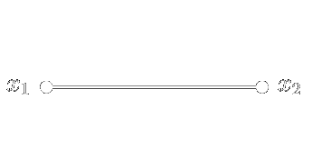
Figure 5: The cluster graph for the NTK.
According to Lemma 1, with \(k=1\) and \(F(\vec{x})\) equal to the NTK, the derivative of
the NTK also scales at most as \(\mathcal{O}(n^0)\). To find the exact scaling, we expand
out the expression for the derivative of the NTK with MSE loss, yielding
with cluster graph shown in Figure 6. This has \(n_e=0, n_o=2, m=4\), and \(s_c=-1\). Thus the derivative of the NTK scales as \(\mathcal{O}(n^{-1})\). If we additionally assume the time-evolved kernel is analytic in the training time \(t\), we can Taylor expand to get the NTK at any value of \(t\),
\[\begin{equation} \mathbb{E}_\theta \left[ \Theta(t)-\Theta(0) \right] = \sum_{k=1}^\infty \frac{t^k}{k!} \mathbb{E}_\theta \left[\frac{d^k\Theta(0)}{dt^k} \right] \sim \mathcal{O}(n^{-1}), \end{equation}\]where we assume we can exchange the Taylor expansion in time with the large-\(n\) limit, and have applied Lemma 1 for all values of \(k\) to the terms in the expansion. The NTK is thus constant during training in the large-\(n\) limit, with corrections scaling as \(\mathcal{O}(n^{-1})\).
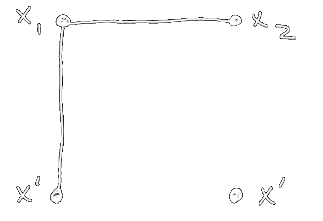
Figure 6: The cluster graph for Eq. \eqref{eq:NTK_td}.
Finite-n Corrections to Training Dynamics
To make progress on deriving the \(\mathcal{O}(n^{-1})\) correction to the network function evolution, we first define the functions \(O_1(x) \equiv f(x)\) and
\[\begin{equation} \label{eq:Os_def} O_{s}(x_1,\ldots,x_{s}) \equiv \sum_{\mu} \frac{\partial O_{s-1} \left( x_1,\ldots,x_{s-1} \right)}{\partial\theta_{\mu}} \frac{\partial f(x_{s})}{\partial\theta_\mu}\,, \quad s \ge 2 \,. \end{equation}\]It is easy to check that, for the case of MSE loss
\[\begin{equation} \label{eq:Os_d_def} \frac{dO_s(x_1,\ldots,x_{s})}{dt} =-\sum_{(x',y')\in D_{\textrm{tr}}} O_{s+1} \left( x_1,\ldots,x_{s},x' \right) \left( f(x')-y'\right) \,, \quad s \ge 1 \,. \end{equation}\]For example, \(O_2\) is the NTK \(\Theta\), and we computed \(d \Theta/dt\) in Eq. \eqref{eq:NTK_td}.
Eqs. \eqref{eq:Os_def} and \eqref{eq:Os_d_def} define an infinite tower of first-order ordinary differential equations (ODEs), the solution to which gives the time evolution of the network function and the NTK.
\[\begin{align} \frac{df(x_1;t)}{dt}&= -\sum_{(x,y)\in D_{\textrm{tr}}}\Theta(x_1,x;t)\left( f(x;t)-y \right)\label{eq:f_ODE}\\ \frac{d\Theta(x_1,x_2;t)}{dt}&= -\sum_{(x,y)\in D_{\textrm{tr}}}O_3(x_1,x_2,x;t)\left( f(x;t)-y \right)\label{eq:NTK_ODE}\\ \frac{dO_3(x_1,x_2,x_3;t)}{dt}&= -\sum_{(x,y)\in D_{\textrm{tr}}}O_{4}(x_1,x_2,x_3,x;t)\left( f(x;t)-y \right)\label{eq:O3_ODE}\\ &\vdots\nonumber \end{align}\]However, solving this infinite tower is infeasible. To proceed, the authors show that the \(O_s\) scale as
\[\begin{equation} \mathbb{E}_\theta \left[ O_{s}(x_1,\ldots,x_s;t) \right] = \left\{\begin{array}{ll} \mathcal{O}\left(n^{1-s/2}\right)&,\ s\, \textrm{even}\\ \mathcal{O}\left(n^{1/2-s/2}\right) &,\ s\, \textrm{odd} \end{array}\right.\, \end{equation}\]and write each \(O_s\) as an expansion in terms of its scaling behavior:
\[\begin{equation} \begin{split} f(x_1;t)&=f^{(0)}(x_1;t)+f^{(1)}(x_1;t)+\mathcal{O}(n^{-2}) \\ \Theta(x_1,x_2;t)&=\Theta^{(0)}(x_1,x_2;t)+\Theta^{(1)}(x_1,x_2;t)+\mathcal{O}(n^{-2})\\ O_3(x_1,x_2,x_3;t)&=O_3^{(1)}(x_1,x_2,x_3;t)+\mathcal{O}(n^{-2})\\ O_4(x_1,x_2,x_3,x_4;t)&=O_4^{(1)}(x_1,x_2,x_3,x_4;t)+\mathcal{O}(n^{-2})\\ O_5(x_1,x_2,x_3,x_4,x_5;t)&=\mathcal{O}(n^{-2})\\ &\quad\!\!\!\vdots \end{split} \end{equation}\]where \(O_s^{(r)}\) captures the \(\mathcal{O}(n^{-r})\) evolution of \(O_s\). This expansion lets us solve the ODEs order by order in \(1/n\), and we show how to calculate the first, \(\mathcal{O}(n^{-1})\) correction. The resultant expressions are unwieldy, so we do not reproduce them here, but refer the reader to Appendix E.4.1 of the paper.
When calculating the \(\mathcal{O}(n^{-1})\) correction, we can ignore all terms of \(\mathcal{O}(n^{-2})\) and higher. In particular, the \(O_s\) ODEs vanish at \(\mathcal{O}(n^{-1})\) for \(s \geq 5\) since \(O_5 \sim \mathcal{O}(n^{-2})\). In addition
\[\begin{equation} \frac{dO_4(x_1,x_2,x_3,x_4;t)}{dt} = \frac{dO_4^{(1)}(x_1,x_2,x_3,x_4;t)}{dt} \sim \mathcal{O}(n^{-2}) \end{equation}\]so we can set \(O_4(t) = O_4^{(1)}(t) = O_4^{(1)}(0)\), which we can compute at initialization.
We first need to solve the \(O_3\) ODE, Eq. \eqref{eq:O3_ODE}, at order \(\mathcal{O}(n^{-1})\), which reads, in integral form
\[\begin{equation} O^{(1)}_{3}(x_1,x_2,x_3;t)=O_3 (x_1,x_2,x_3;0)-\int_{0}^{t}dt^{\prime} \!\!\sum_{(x,y)\in D_{\textrm{tr}}}O_4^{(1)} (x_1,x_2,x_3,x;0)\left(f^{(0)}(x;t')-y\right). \end{equation}\]We substitute \(f^{(0)}(x;t')\) and the initial value \(O_4^{(1)}(t=0)\) into this equation, where \(f^{(0)}(t)\) is given by the solution to Eq. \eqref{eq:f_ODE} at leading order:
\[\begin{align} f^{(0)}(t) &= y + e^{-t \Theta_0} \left(f_0 - y \right) % \Theta^{(0)}(t) &= \Theta_0 \end{align}\]After performing the integral over \(dt'\), we obtain a closed-form expression for \(O_3^{(1)}(x_1,x_2,x_3;t)\).
Next we solve the \(\Theta\) ODE, Eq. \eqref{eq:NTK_ODE}. The NTK is constant during training at \(\mathcal{O}(n^0)\), so
\[\begin{equation} \Theta(x_1,x_2;t)=\Theta^{(0)}(x_1,x_2;0)+\Theta^{(1)}(x_1,x_2;t), \end{equation}\]and the \(\Theta\) ODE reads, in integral form
\[\begin{equation} \Theta^{(1)}(x_1,x_2;t) = -\int_{0}^{t}dt^{\prime}\!\!\sum_{(x,y)\in D_{\textrm{tr}}}O^{(1)}_{3}(x_1,x_2,x;t')\left(f^{(0)}(x;t')-y\right) \,. \end{equation}\]After plugging in \(f^{(0)}(x;t')\) and our previously obtained expression for \(O_3^{(1)}(x_1,x_2,x_3;t')\), performing the \(dt'\) integral yields a closed-form expression for \(\Theta^{(1)}(x_1,x_2;t)\).
Finally, we solve the \(f(x;t)\) ODE, Eq. \eqref{eq:f_ODE}:
\[\begin{equation} \frac{df(x;t)}{dt}=-\!\!\sum_{(x',y')\in D_{\textrm{tr}}} \left(\Theta(x,x';0)+\Theta^{(1)}(x,x';t)\right) \left(f(x';t)-y'\right)+\mathcal{O}(n^{-2}) \end{equation}\]Plugging in \(f^{(0)}(x;t')\) and our result for \(\Theta^{(1)}(x_1,x_2;t')\) yields a final closed-form expression for \(f(x;t)\) that includes the \(\mathcal{O}(n^{-1})\) correction.
Discussion and Conclusions
Using Feynman diagrams to keep track of the terms in correlation functions allows us to quickly identify how a correlation function scales with \(n\). For correlation functions with derivative tensors — which appear in the analysis of the NTK and its derivatives — the scaling is given by the properties of a simple graph defined in Conjecture 1. By knowing the scaling of the NTK and its derivatives, we can organize the equations defining the evolution of the network function and NTK as an expansion in \(1/n\), which can then be solved order-by-order in \(1/n\). We showed how to calculate the \(\mathcal{O}{(n^{-1})}\) correction, but the procedure can be carried out to arbitrary order in \(n\). This opens the way for using the NTK to describe the evolution of finite-width networks during training.